Editor’s Note: Yes, I know, you have questions. Why Am I posting here? Well, all I can say is that life happens. I will write a fuller post on future plans once I’m actually back fully from the Holidays but the short of it is, I will be posting more out of here in the near future. Never fear though, I have plans to keep writing until they pry the keyboard from my cold dead hands (or someone writes a large check!). Now, I give you a long delayed post, how does the new metric I used for the season previews work exactly?
“It is common sense to take a method and try it: If it fails, admit it frankly and try another. But above all, try something.”
-Franklin Delano Roosevelt, Oglethorpe University Commencement Address (22 May 1932)
We did worse last year at predictions than we have in previous years. I can freely admit it. Now, I could have taken my spreadsheets and gone on home or I could have rebuilt everything from the ground up stronger and better than before.
Much like the Spurs last season, failure just served as fuel for this offseason.
The results of that effort are collected here for your easy reference:
Let’s talk a bit about the journey though.
One of the more interesting about models is that a descriptive metric is not necessarily a predictive metric. This point was analysed at length by Alex Konkel. Wins Produced was designed as a descriptive metric and not a predictive one. It is very good at doing what it was designed for and that is determining what the players actually did in a season and their relative value. However when it comes to predictive ability it tends to lag behind as constructed.
That’s the list of internet wide predictions on Win Totals for the past two NBA seasons. You’ll note that the Wins Produced predictive models I put together come out with an RSME of 7.6 for 2013 and 10.65 in 2014 versus a best of 5.9 and 8.1 respectively.
What this basically told me, Is that I needed to build a new predictive metric.
Luckily, I already had the outline of one in my mind. Let’s go on a tangent for a bit. Don’t worry though, it’s important to the story.
One of the recurring ideas of my writing on the internet has been the goal of continuing to grow the existing boxscore based models. I’ve always wanted to be able to look at game to game and even play by play data using the same concepts and base equation that Prof. Berri outlined in his work:
Here is the specific model linking winning percentage to offensive and defensive efficiency.
- The model was estimated with data from 1987-88 to 2010-11
- Data taken from Basketball Reference
- Dependent Variable is Winning Percentage
Independent Variable Coefficient t-statistic Offensive Efficiency 3.152 82.110 Defensive Efficiency -3.134 -73.348 Constant term 0.481 8.702 Adjusted R2 = 0.94
Where
- Offensive Efficiency = Points Scored divided by Possessions Employed (PE)
- Defensive Efficiency = Points Surrendered divided by Possessions Acquired (PA)
and
- PE = FGA + 0.45*FTA + TO – REBO
- PA = DFGM + 0.45*DFTM + REBD + DTO + REBTM
FGA = Field Goal Attempts FTA = Free Throw Attempts TO = Turnovers REBO = Offensive Rebounds DFGM = Opponent’s Field Goals Made DFTM = Opponent’s Free Throws Made REBD = Defensive Rebounds DTO = Opponent’s Turnovers REBTM = Team Rebounds The formulation for PE and PA is explained in Berri (2008).
The value for FTA and DFTM is explained in Berri (2008)
REBTM refers to Team Rebounds that change possession. This calculation is detailed in Berri (2008)
Dave took this model and used the season total data to build a robust explanatory model. However, because of the way it was built there was data that was lost in the translation. There was granularity that was simply not readily available at the time. Using season as opposed to game data forced some compromises. Defense outside of the boxscore was considered wholly as a team activity.The detail of where the actual value was coming from was a submerged in the one number. Team adjustments were required for defense and other activities and while mathematically sound, reasonable and backed by the actual empirical data, they led to countless discussions because of their complexity.
I had decided early this offseason that this was the summer I build my game metric. I wanted to build something simple, based on sound principles and intuitive. To that end, I based everything around Win Score. What I was surrendering in mathemathical complexity, I was expecting to gain back in the order of magnitude increase in granularity by going from season totals to a game to game tally. I was not disappointed.
- Win Score = Points + Steal + Offensive Rebounds + 0.5*(Defensive Rebounds +Assists + Blocks) – Turnovers – Field Goal Attempts – 0.5*(Free Throw Attemps + Personal Fouls)
- if player A has a Win Score of 10 in 40 minutes played at center and the opposing team’s Centers produce a Win Score of 8 for the game, Player A’s Opponent Adjusted Win Score per 48 (OAWS P48) is equal to : 10*(48/40) – 8= 4.
As an example for a player playing multiple positions in a single game (e.g. 50% PF and 50% C) the calculation would look something like this :
OAWS/48 = [Win Score] * (48/[Minutes Played]) – [Opponent Win Score at Position 1] * [Time at Position 1]/48 – [Opponent Win Score at Position 2] * [Time at Position 2]/48
Q: What is Marginal Win Score per 48 (MWS48)?
Marginal Win Score per 48 is the basketball metric I use to attribute wins and losses to individual players on any given basketball team. It is based upon the Win Score metric created by economics Professor David Berri and his colleagues who wrote the excellent book The Wages of Wins. Their work uncovered how traditional basketball statistics correlate with wins. Win Score is simply an expression of their findings, and Marginal Win Score is derived from that.
…………..
Q: How does Marginal Win Score differ from Win Score?
Its basically a comparative difference.
Win Score attributes wins to players by comparing their Win Score per 48 (WS48) to the NBA average WS48 at the player’s position. Marginal Win Score attributes wins produced on the basis of the Player’s Win Score and the Win Score he and his team allow opponents who play the same position to produce.
The reason I prefer this method is simple. No team and no individual player ever competes against “the average”. They compete against actual opponents. And in the game of basketball, one can impact the level of efficiency one’s opponents are able to achieve (I am loosely referring, of course, to “defense”). That fact has to be recognized, I believe, in any win calculation.
………..
Q: So Marginal Win Score is Win Score with defense?
Yes and no. Basketball defense is so intertwined between the individual and the team, its impossible to precisely value each player’s defense. So that’s not what I’m claiming to do. Instead what I like to say is “With Marginal Win Score each team and each player on that team produces wins based upon a comparison between his positional Win Score and the Win Score average that he and his team allow at his given position“. Is defense part of that? Yes. Can individual defensive effort effect that? Yes. But are there elements of that defense that are not in each player’s control? Yes.
That’s why I don’t claim that “Marginal Win Score” is necessarily about defense per se. Because basketball defense is partially an individual act, and partially a team act. And since its really a poorly compensated act, it relies somewhat on the cooperation and collective morale of the entire team.
Therefore a player’s Marginal Win Score will be effected by elements out of his control. A player on a hopeless team whose teammates play no defense has little to no incentive to play defense himself. And even if he does, how is he going to stop his counterparts alone? So you have that element.
But I’m comfortable with that, because, really, that is what winning in sports is all about. You’re not always faced with ideal circumstances or circumstances that are 100% under your control. Producing wins, or more precisely, performing the acts that produce wins, is often circumstantial. That’s just sports.
A few more bits of math are needed. The correlation (r-square) between OAWS and actual point margin on a game to game basis is 92% from the 1986 to 1987 season. This is functionally the same as the result if we did the same for the full wins produced model.
Next, I have to work out the correlation of OWAS per game to actual point margin per game. I did this on a season to season basis. The conversion factor from OWAS to Point Margin is listed in the table below:
| Season | Conversion from OAWS to Point Margin Produced |
| 1987 | 59.2% |
| 1988 | 59.0% |
| 1989 | 59.7% |
| 1990 | 60.8% |
| 1991 | 60.0% |
| 1992 | 60.0% |
| 1993 | 59.6% |
| 1994 | 59.4% |
| 1995 | 60.0% |
| 1996 | 61.4% |
| 1997 | 60.5% |
| 1998 | 61.0% |
| 1999 | 60.3% |
| 2000 | 60.9% |
| 2001 | 61.1% |
| 2002 | 62.6% |
| 2003 | 62.4% |
| 2004 | 60.2% |
| 2005 | 61.2% |
| 2006 | 61.9% |
| 2007 | 61.7% |
| 2008 | 62.2% |
| 2009 | 61.8% |
| 2010 | 61.5% |
| 2011 | 61.0% |
| 2012 | 63.7% |
| 2013 | 62.4% |
| 2014 | 62.5% |
Using this conversion factor I can create Point Margin Produced (PMP) simply as OAWS times 62.5% for 2014 for example. I can then map that to a few familiar formats:
- Game Wins Produced per 48 (GWP48) = PMP per 48/31.1 + 48*1230/(Minutes for season)
- Game Wins Produced= Game Wins Pruduced per 48 times Player MP /48
At this point the basic model is done. However, due to the nature of scorekeeping in the NBA we have certain events that are not directly attributed to actual players but to the teams themselves, team rebounds and team turnovers. These are actually fairly hard to dig out and almost impossible to asign to any one player. Not accounting for them causes error between the projected point margin in a game and the actual point margin. This is easy enough to calculate. That difference, which is coming from the team assigned stats, forms the basis of the team adjustment ( take the difference in the point margin tabulated for each game and divide it up by minutes). Adding that in gives us correlation similar to what I’ve previously observed from doing Wins Produced on a game to game basis. However, it’s not an adjustment that we strictly need.
The end result looks like this:
Wins Produced versus Games Wins Produced for 2014
You’ll note that some players that are recurring sources of arguments here, such as Melo and Aldridge, benefit from the change. We will be talking about this more during the season. A few more notes:
- The more minutes a player plays, the more accurate the number is. A player playing point guard for 400 minutes next to Chris Paul will see a significant benefit to his defensive and offensive numbers. The next level (play by play) will address that in the future.
- The metric can be divided into the following components:
1. Scorer Point Margin per 48: ((Points – Field Goal Attempts – 0.5*(Free Throw Attemps ) – Average at Position) times the conversion factor : Simple measure of how good/bad a player is at scoring
2. Handle Point Margin per 48: ((.5*Assists– Turnovers )- Average at Position) times the conversion factor: Simple measure of how good/bad a player is at handling the ball.
3. Rebounding Point Margin per 48: ((Offensive Rebounds + 0.5*Defensive Rebounds) – Average at Position) times the conversion factor: Simple measure of how good/bad a player is at getting rebounds.
4. Defensive Point Margin per 48: ((Steal + 0.5*Blocks – .5*Personal Fouls + Opponent_Difference_from_Average_WS_Production)- Average at Position) times the conversion factor: Simple measure of how good/bad a player is at Defense. Two components here: Box Score Defensive Point Margin per 48 or defense as measured in the Boxscore and Opponent based Defensive Point Margin or how much more or less production we see from the player’s average opponent.
5. Finally the team component which is just the differential on a game to game basis divided on a per minute basis.
Here’s a look at the R-Square for different components of the metric to actual team point margin per game:

You’ll note that the team adjustment is mostly unnecessary. Just the player attributed boxscore stats give you an R-squared of 97%. Interestingly, the just scoring and boxscore defense gives you around 90% of all the information you need.
Let’s get back on track. With the new metric in hand,I did some testing (yes it’s show my work time).
- Wins Produced and Wins Produced per 48
- Raw Wins Produced and ADJP48 (i.e Wins Produced with no position adjustment)
- Game based wins produced without any team adjustment. Basically, I just used the player boxscore and opponent stats and ignored everything else.
- Game based wins produced with the team adjustment. .
- Total model Wins for each model versus actual wins for the year (descriptive)
- Retrodiction test for teams. Predicted wins based on Prod per 48 for players the previous season and actual minutes for that season. I put a minute floor of 400 for the previous and current season. Player’s below that floor just saw their actual win totals. (Predictive)
- Year to Year variation in productivity per 48 with the same minute cap. All players.
- Year to Year variation in productivity per 48 with the same minute cap. Players who did not change teams.
- Year to Year variation in productivity per 48 with the same minute cap. Players who did change teams


Let’s recap:
- I built a new game metric (OAWS, PMP, Game Wins Produced) based on Wins Produced principles and it was good.
- I rebuild the projection model from the ground up. I tested multiple metrics and the new game metric was the best. There is a simple version of the Age model and a game to game team correction included in the metric.
- For rookies and euro’s I used and adapted the existing draft models (see here).
So all the projection articles for this season when talking about Wins Produced and WP48 are talking about Game Wins Produced and Game WP48 using the team adjustment as defined in this article.
With the metric in hand, I went to do the season simulation or as the Andres calls it: the minute projection death trap. Again, I was up to facing the impossible challenge. The key was this little tidbit:
| Minute Map | Depth Chart Current Season | Depth Chart Current Season | Depth Chart Current Season | |
| Age Group | Depth Chart Previous Season | 1 to 5 | 6 to 10 | 11 & Up |
| 18 to 22 | 1 to 5 | 62% | 25% | 13% |
| 18 to 22 | 6 to 10 | 23% | 46% | 31% |
| 18 to 22 | 11 & Up | 5% | 21% | 74% |
| 23 to 25 | 1 to 5 | 64% | 26% | 10% |
| 23 to 25 | 6 to 10 | 26% | 43% | 31% |
| 23 to 25 | 11 & Up | 9% | 23% | 68% |
| 26 to 29 | 1 to 5 | 69% | 25% | 6% |
| 26 to 29 | 6 to 10 | 37% | 41% | 22% |
| 26 to 29 | 11 & Up | 15% | 39% | 46% |
| 30 and up | 1 to 5 | 74% | 20% | 6% |
| 30 and up | 6 to 10 | 31% | 46% | 23% |
| 30 and up | 11 & Up | 16% | 39% | 45% |
That table represents a map of a players motion on the depth chart as a function of age and their place in the depth chart the previous season. Using this, the players average minutes over the last three season, their minute variability, their projected place on the depth charts, teams minute allocation patterns and a lot of random functions, I was able to build a minute allocation simulation for each team. I then combined that with expected average production for each player as well as the error for each projections (and of course more random number generator functions).
Finally, I identified the typical error introduced by the schedule and Home Court (it’s around 2.1 wins and completely random season to season) and threw that in together with corrections to make sure that the wins for the league add up to 1230 for each simulation.
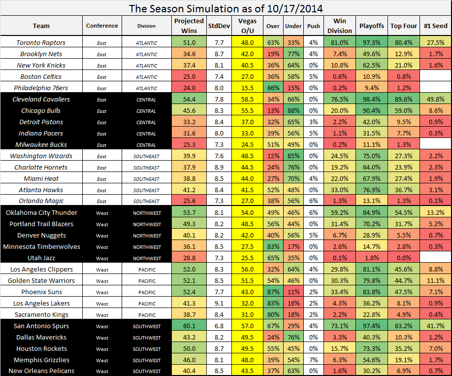
The result of course, is your season projections for each team.
As you have already seen.
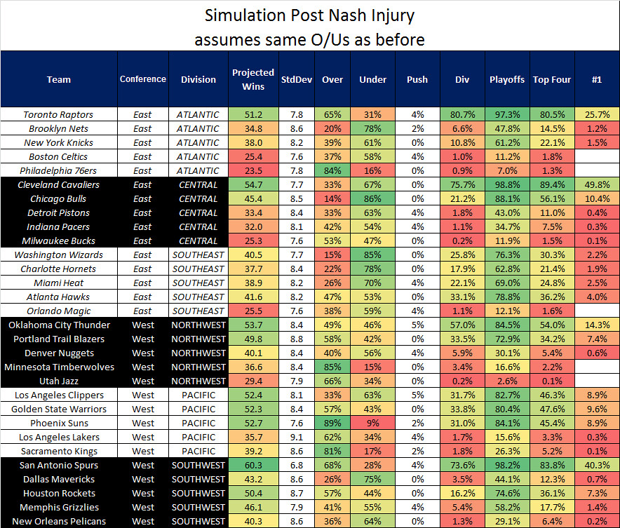
Still here? It occurs to me that the rosters have changed a tiny bit since 10/17 when I locked in the simulation. In particular, Steve Nash is out.
Are you ready for some basketball?
-Arturo


January 5th, 2015 → 16:13
[…] The tools in this post are all based on the game based metric that I explained in detail here. […]
January 7th, 2015 → 17:18
[…] is a fabulous idea. It just so happens that I have a metric that keeps track of every single game (explained in detail here) that assigns a score to each and every player. If I take my metric tracking file and add in a […]
January 13th, 2015 → 13:38
[…] league. Given that it just so happens that I have a metric that keeps track of every single game (explained in detail here) and assigns a score to each and every player, creating a tool for and keeping track of the Wilt is […]